Sato-Tate Distributions
Abhiram Kidambi (MPI MIS and AEI Potsdam)
Slides available at: abhirammk.github.io/talks/satotate
Overview of the talk
I was asked to give a pedagogical introduction to the Sato-Tate conjecture assuming limited background in number theory and arithmetic geometry.
- Example 1: The Ramanujan discriminant function (This is a remarkably important function in mathematics!)
- Example 2: Polynomial roots and the Chebotarev density theorem
- Zeta functions and their arithmetic
- Elliptic curves over \mathbb{Q}
- Sato-Tate distribution and conjecture for elliptic curves
- Generalizing Sato-Tate conjectures
Notation
- \mathbb{H}:= \{ a + i b | a \in \mathbb{R}, b \in \mathbb{R}_{>0} \}
- z \in \mathbb{H}
Ramanujan Discriminant \Delta
Consider the Ramanujan discriminant function \Delta(z) = q \prod_{n=1}^\infty (1-q^n)^{24}, \ q:= \exp(2\pi i z)
Taylor expand \Delta(z) around q =0 (i.e. Fourier expand) as \displaystyle \Delta(z) = \sum_{n=1}^\infty \tau(n)q^n to see: \Delta(z) = q - 24 q^2 + 252 q^3 - 1472 q^4 + 4830 q^5 - 6048 q^6 - 16744 q^7 + O(q^8) Ramanujan studied the coefficients \tau(n) and made the following observations:
- Multiplicativity: \tau(m\cdot n) = \tau(m)\tau(n) if (m,n)=1
- Ramanujan Conjecture: |\tau(p)| \leq 2 p^{11/2} for p prime (Proof in Deligne (1980))
The Ramanujan conjecture is the precursor to first instance of the Sato-Tate conjecture
Arithmetic of divisors of integers
The Ramanujan conjecture at first glance suggests that there is no control over the sign of \tau(p). How does one quantify that?
Let \displaystyle \sigma_k(n) := \sum_{d|n} d^k be the divisor sigma function. Example: \sigma_2(8) = 1^2 + 2^2 + 4^2 + 8^2 = 85
What are the generating functions for \sigma_k(n)? Eisenstein series E_{k+1}(z).
\ E_4(z) = 1 -\frac{8}{B_4} \sum_{n=1}^\infty \sigma_3(n) q^n, \ \ E_6(z) = 1 -\frac{12}{B_6}\sum_{n=1}^\infty \sigma_5(n) q^n
\text{Infact: } \Delta(z) := \frac{E_4(z)^3 - E_6(z)^2}{1728} = \sum_{n=1}^\infty \tau(n) q^n, \ \ 1728\cdot \tau(n) = C_3^4(n) - C_2^6(n) \text{where } C_m^k(n) = \sum_{j=1}^m {m \choose j} \left [ \sum_{\substack{m_1,\cdots,m_j > 0 \\ m_1 + \cdots + m_j = n}} \sigma_{k-1}(m_1)\cdots \sigma_{k-1}(m_j)\right] C_m^k(n) is the n^{th} coefficient of E_k(z)^m. B_i is the i^{th} Bernoulli number.
Randomness in the coefficients of \Delta(z)
- For \displaystyle E_k(z) = 1 - \frac{2k}{B_k}\sum_{n=1}^\infty \sigma_{k-1}(n) q^n, the p^{th} coefficient \displaystyle C_1^k(p) \approx \frac{-2k}{B_k}p^{k-1} for p prime.
- We don’t care much about composite n since \displaystyle |C_1^k(p_n)| > |C_1^k(n)| where p_n is the smallest prime greater than n.
- The sign of the coefficients are fixed, and E_k has polynomial grown in coefficients as O(p^{k-1}).
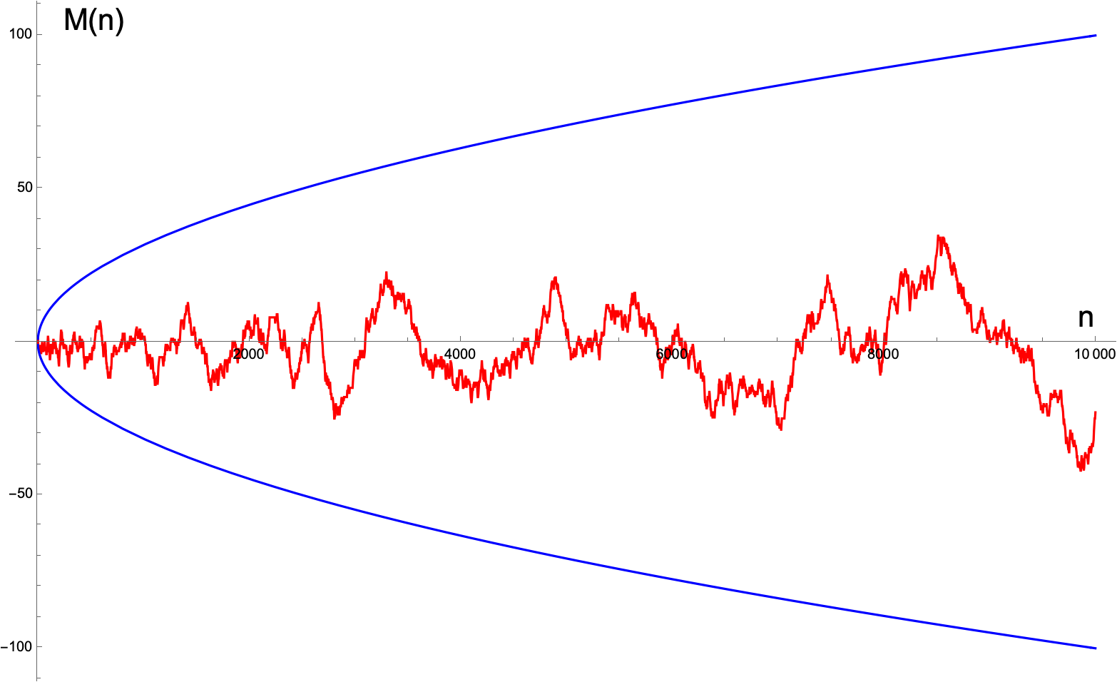
- But what about \tau(n)= C_3^4(n) - C_2^6(n)? Let \displaystyle M(\tau(n)):= \sum_{m=1}^n \mathrm{sgn}(\tau(m)).
- Open Conjecture (Lehmer (1947)): There is no n\in \mathbb{Z}_{>0} such that \tau(n) = 0.
Current known estimates: \tau(n) \neq 0 for upto n \approx 8 \cdot 10^{23} (Derickx, Hoeij, and Zeng (2013)). - So what does the function M(\tau(n)) look like?
Graph of M(\tau(n))
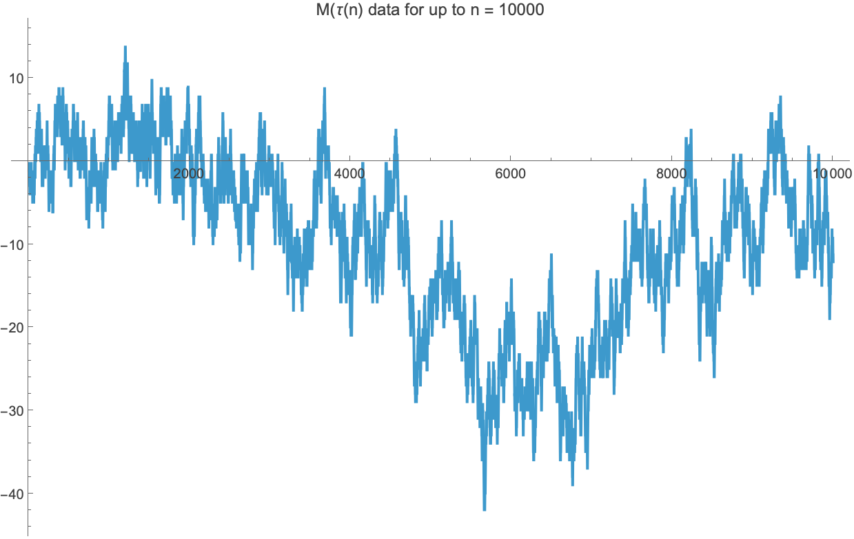
This looks resembles a random Browninan motion and resembles the graph of the Mertens function.
This graph demnonstrates a randomness in the sign of the coefficients of the \Delta(z) function.
But what about normalized bounds?
Ramanujan Conjecture/Deligne Theorem: |\tau(p)| \leq 2 p^{11/2} \iff x_p := \dfrac{\tau(p)}{2 p^{11/2}} \in [-1,1].
So how is x_p distributed in [-1,1]?
The Horizontal Sato-Tate distribution for x_p
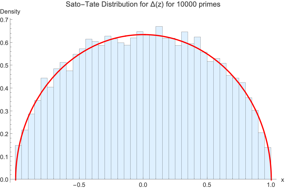
On the left: Distribution for x_p for 10000 primes
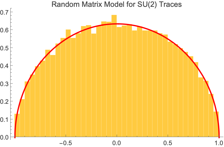
On the right: Distribution eigenvalues of an ensemble of 10000 random SU(2) matrices
Life advice:
When you are given a number, ask if it arises as a polynomial root or value of an integral or a value of a nice (read: special/algebraic/transcendental) function.
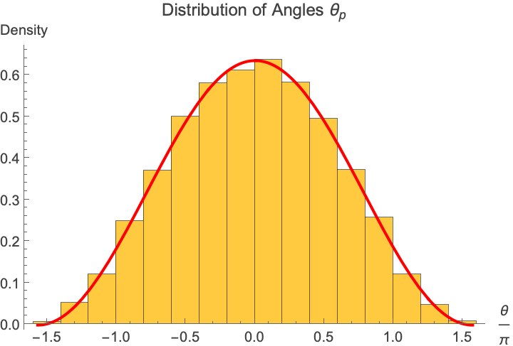
Angular distributions
Let x_p =: \sin(\theta_p) \Rightarrow \theta_p := \arcsin(x_p). How is \theta_p distributed?
Example 2: Distribtion of Polynomial Roots
- Let f(x) \in \mathbb{Z}[x] be a polynomial with no repeating roots (i.e. \mathrm{disc}_{\mathbb{A}}(f) \neq 0).
- Generically, given an arbitrary polynomial of degree d in variables x_1,\cdots,x_n, there is no algorithm to determine if whether this polynomial has \mathbb{Q} solutions. [Undecidability of Hilbert’s 10th problem by Matiyasevich, Robinson, David and Putnam (MRDP Theorem)].
- But one can find solutions over \mathbb{F}_p.
- Let f_p(x) = \bmod (f(x),p) \in \mathbb{Z}/p\mathbb{Z}[x] \simeq \mathbb{F}_p[x]
- Let N(f,p) := \#\{ x\in \mathbb{F}_p | f_p(x) \cong 0 \bmod p\}.
- Question: For a fixed f(x) how does N(f,p) vary with p?
Let us consider two examples. First, let f(x) = x^3 - x + 1,\ \mathrm{disc}_{\mathbb{A}}(f) = -23:
| p | 2 | 3 | 5 | 7 | 11 | 13 | 17 | 19 | 23 | 29 | 31 | 37 | 41 | 43 | 47 | 53 | 59 | 61 | 67 | 71 |
|---|---|---|---|---|---|---|---|---|---|---|---|---|---|---|---|---|---|---|---|---|
| N(f,p) | 0 | 0 | 1 | 1 | 1 | 0 | 1 | 1 | 2 | 0 | 0 | 1 | 0 | 1 | 0 | 1 | 3 | 1 | 1 | 0 |
Can you spot a pattern?
Ratios
For all primes p \leq B, let \displaystyle c_i(B) := \frac{\#\{ p\leq B | N(f,p) = i \}}{\pi(B)}. Recall that \pi(x) = \#\{p \leq x\}.
So let’s compute this. Let again f(x) = x^3 -x+1.
| B | c_0(B) | c_1(B) | c_2(B) | c_3(B) | ||
|---|---|---|---|---|---|---|
| 10^3 | 0.3273810 | 0.5178571 | 0.005952381 | 0.1488095 | ||
| 10^4 | 0.3319772 | 0.5101709 | 0.0008136697 | 0.1570382 | ||
| 10^5 | 0.3337156 | 0.5028148 | 0.0001042535 | 0.1633653 | ||
| 10^6 | 0.3331932 | 0.5007771 | 0.0000127391 | 0.1660170 | ||
| 10^7 | 0.3333614 | 0.5002656 | 0.0000015047 | 0.1663715 | ||
| 10^8 | 0.3333366 | 0.5000582 | 0.0000001735 | 0.1666050 |
Theorem: For equations like f(x) above, c_0 \sim \frac{1}{3}, c_1 \sim \frac{1}{2}, c_2 \sim 0, c_3 \sim \frac{1}{6} Meaning: The probabilty of you finding i solutions mod p is c_i.
Chebotarev Density Theorem (K = \mathbb{Q})
Theorem(Chebotarev (1926)): Let L/K be a finite extension of K that is Galois, with a Galois group \mathrm{Gal}(L/K)=: G. Let \sigma_\mathfrak{p} be the Frobenius conjugacy class. For every subset C of G stable under conjugation, we have \lim_{B\rightarrow \infty} \frac{\{\mathfrak{p} \subseteq \mathcal{O}_K | N(\mathfrak{p}\leq B), \sigma_{\mathfrak{p}\subseteq C}\}}{\{\mathfrak{p} \subseteq \mathcal{O}_K | N(\mathfrak{p}\leq B)\}} = \frac{|C|}{|G|} Note: The Frobenius conjugacy class captures how primes in K that split in L are related to each other in the Galois group.
For f(x) = x^3 - x + 1, G = S_3, |G| = 6. There are 3 conjugacy classes (A_{0,1,3}) of S_3 of trace 0,1,3.
A_0 = \begin{pmatrix} 0&1&0 \\ 0&0&1 \\ 1&0&0 \end{pmatrix}, \begin{pmatrix} 0&0&1 \\ 1&0&0\\ 0&1&0 \end{pmatrix}, \ \ A_1 = \begin{pmatrix} 1&0&0\\ 0&0&1 \\ 0&1&0 \end{pmatrix}, \begin{pmatrix} 0&0&1 \\ 0&1&0 \\ 1&0&0 \end{pmatrix}, \begin{pmatrix} 0&1&0 \\ 1&0&0 \\ 0&0&1 \end{pmatrix}, \ \ A_3 = \begin{pmatrix} 1&0&0 \\ 0&1&0 \\ 0&0&1 \end{pmatrix}
This gives: |A_0| = 2, |A_1| = 3, |A_3|= 1.
Therefore c_i = \frac{|A_i|}{|G|} which gives c_0 = \frac{1}{3}, \ c_1 = \frac{1}{2}, \ c_3 = \frac{1}{6}
A second polynomial example
Now let g(x) = x^3 + x. The Galois group of this polynomial is S_2 of order 2, which has two, order 1 conjugacy classes:
A_1 = \begin{pmatrix} 0&1 \\ 1&0 \end{pmatrix}, \ A_3 = \begin{pmatrix} 1&0\\ 0&1 \end{pmatrix}
Applying the Chebotarev density theorem, we see that c_1 = \frac{1}{2} \ c_3 = \frac{1}{2}.
Note: The trace/cycle length interpretation is not the valid here. Here we are concerned with primes that are congruent to either 1 or 3 mod 4
Comparing with empirical data:
| B | c_0(B) | c_1(B) | c_2(B) | c_3(B) | ||
|---|---|---|---|---|---|---|
| 10^3 | 0 | 0.5178571 | 0.005952381 | 0.4761905 | ||
| 10^4 | 0 | 0.5036615 | 0.0008136697 | 0.4955248 | ||
| 10^5 | 0 | 0.5012510 | 0.0001042535 | 0.4986447 | ||
| 10^6 | 0 | 0.5009300 | 0.0000127391 | 0.4990573 | ||
| 10^7 | 0 | 0.5001633 | 0.0000015047 | 0.4998352 | ||
| 10^8 | 0 | 0.5000386 | 0.0000001735 | 0.4999612 |
Why does this happen?
Brief explanation
The Galois group of f(x) = x^3 - x + 1 is S_3 and its representation is 2 dimensional.
The Galois group of g(x) = x^3 + x is S_2 and its representation is 1 dimensional.
When viewed as algebraic varieties of the form X_1:= y^2 = f(x), \ \ T_2 := y^2 = g(x), T_1, T_2 are elliptic curves over \mathbb{Q}.
This phenomenon where the Galois group and representation simplies means that the elliptic curve T_2 has simpler arithmetic, and this is due to the fact that it has a larger endomorphism algebra than T_1.
Philosophically, when algebraic varieties of \dim d try to arithmetically behave like varieties of dimension d', 1\leq d' < d, such varieties have much richer properties.
This is known as complex multiplication.
Zeta functions
Complex analytic functions which capture number of solutions to “polynomial equations”.
Let X be a smooth projective variety over K, \ \mathrm{char}(k) \neq 2. Let K = \mathbb{Q}. For a prime p, Z_X(p,T) := \exp \left( \sum_{n=1}^\infty \frac{N(X,p^n)}{n} T^n\right)
From the Grothendieck-Lefschetz trace formula, N(X, p^n) = \mathrm{Tr}(\rho_X(\mathrm{Frob}_p)^n), where the Frobenius endomorphism on \mathbb{F}_p acts as \mathrm{Frob}_p: \mathbb{F}_p \rightarrow \mathbb{F}_p^n = \mathbb{F}_p[x]/(f(x)), where f(x) is irreducible over \mathbb{F}_p and \deg(f(x)) = n.
Note: The image of \rho_X(\mathrm{Frob}_p) is a element of \mathrm{GL}_d, and the trace of that matrix contains information of the number of solutions N(X,p^n).
\exp \left( \sum_{n=1}^\infty \frac{N(X,p^n)}{n} T^n\right) = \exp \left( \sum_{n=1}^\infty \frac{\mathrm{Tr}(A^n)}{n} T^n\right) = \det(1 - AT)^{-1} \\ \Longrightarrow Z_X(p,T) = \frac{1}{\det(1- \rho_X(\mathrm{Frob}_p)T)}
Properties of zeta functions
For a smooth projective variety X as before, the local zeta function for p prime satisfies the following (originally conjectured by Weil (1949)):
\displaystyle Z_X(p,T) = \frac{P_1(T)P_3(T)\cdots P_{2d-1}(T)}{P_0(T)P_2(T)\cdots P_{2d}(T)}, and P_i(T) \in \mathbb{Q}[T].
If p \nmid \mathrm{disc}(X), then \deg (P_i(T)) = b_i
The roots of P_i(T) are the same as the roots of \displaystyle T^{b_{2d-i}} P_{2d-i}\left(\frac{1}{p^d T}\right). This follows from the functional equation Z_X(p,T) = \pm p^{-\frac{n\chi}{2}} T^{-\chi}Z_X\left(\frac{1}{p^d T}\right)
The roots of P_i(T) are complex numbers whose absolute value if p^{i/2}.
Proofs: (1,2): Dwork (1960), (3): Grothendieck (1964), (4): Deligne (1974)
Elliptic curves over \mathbb Q
- An elliptic curve has b_0 = b_2 = 1, \ \ b_1 = 2.
- Over fields K such that \mathrm{char}(K)\neq 2, the elliptic curve admits the form
X:= y^2 = x^3 + ax + b, \ a,b \in \mathcal{O}_K. (For K =\mathbb{Q}, \mathcal{O}_K = \mathbb{Z}) - \mathrm{disc}(X) = -16(4a^3 + 27b^2)
For a prime p\nmid \mathrm{disc}(X), the local zeta function of the elliptic curve is
Z_X(p,T) = \frac{1- a_p T + pT^2 }{ (1-T)(1-pT)} = \exp \left( \sum_{n=1}^\infty \frac{N(X,p^n)}{n} T^n\right)
- If we Taylor expland both the terms wrt T around 0, we find \#(N(X,p)) = p + 1 - a_p
- Deligne (1974): the absolute value of the roots of 1- a_p T + T^2 should be p^{1/2}
- This gives us the bound |a_p|\leq 2 p^{1/2} i.e. \dfrac{a_p}{2p^{1/2}} \in [-1,1]
Short aside/Big picture
The bound |a_p|\leq 2 p^{1/2} i.e. \dfrac{a_p}{2p^{1/2}} \in [-1,1] looks a lot like the Ramanujan bound from earlier which was proven in Deligne (1980), with the difference being p^{1/2} instead of p^{11/2}.
These are examples of the same phenomenon, known as modularity theorems.
For the case of elliptic curves over \mathbb Q without complex multiplication, we originally were unable to spot patterns in number of solutions since the Galois group was non-abelian.
But the modularity theorem by Taylor and Wiles (1995), Wiles (1995), Breuil et al. (2001) says that for elliptic curves a_p is predictable in terms of the p^{th} Fourier coefficient of a special kind of periodic function, known as newforms
(Holomorphic cuspidal modular forms which are eigenfunctions of every Hecke operator acting on the space of modular forms.)This means that there is a non-abelian reciprocity law which generalizes Gauss reciprocity.
The mathematical program to find general reciprocity laws is known as the Langlands program, and the modularity theorem for elliptic curves is the simplest case of it.
For experts: The case Ramanujan’s conjecture arises from the modularity of a 11 dimensional variety K_{10} which is a fibered product of 10 copies of the unviersal elliptic curve over Y_1(N)
Sato-Tate distribution for elliptic curves
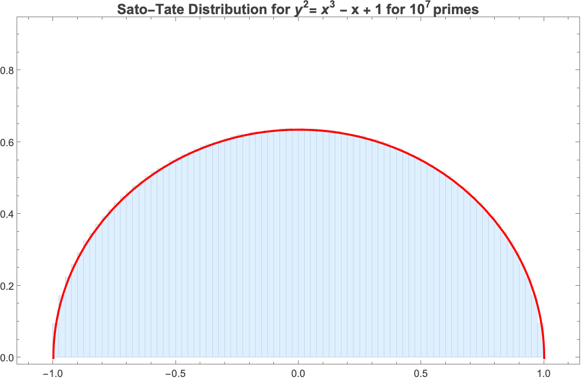
Red line denotes the graph of S(x) = \frac{2}{\pi}\sqrt{1 - x^2}
The Sato-Tate conjecture for elliptic curves
For an embarassingly long time, M. Sato’s contributions were overlooked because of a very Japanese problem - Which Sato was responsible for the computer experiments?!
Conjecture(Sato, Tate (1965)),
Theorem (Taylor (2008), Clozel, Harris, and Taylor (2008), Barnet-Lamb et al. (2011a), Barnet-Lamb et al. (2011b)):
Let E_{\mathbb{Q}} be an elliptic curve without complex multiplication. The sequence \{\frac{a_p}{2\sqrt{p}} \} in the limit p\rightarrow \infty is equidistributed with respect tp the push forward of the Haar measure on \mathrm{SU}(2) i.e., for all [a,b]\subset [-1,1], \lim_{B\rightarrow \infty} \frac{\#\{p\leq B | \frac{a_p}{2\sqrt{p}}\in [a,b] \}}{\pi(B)} = \frac{2}{\pi}\int_{a}^b \sqrt{4-t^2} dt
Sato-Tate for CM elliptic curves
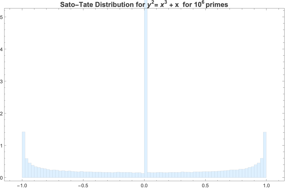
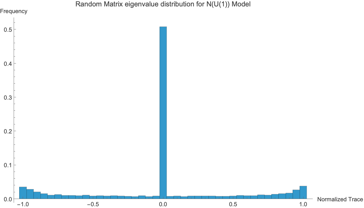
The group wrt which the x_p for X are equidistributed are known as Sato-Tate groups (ST(X)). Sato-Tate groups of X are compact Lie groups containing a dense subset of the image of a Galois representation that maps the Frobenius elements onto its conjugacy classes.
For elliptic curves over K, these are either \mathrm{SU}(2) (no CM), \mathrm{U}(1) (CM defined over K), or \mathrm{N}(\mathrm{U}(1)) (CM not defined over K).
Generalizing Sato–Tate
- Hyperelliptic curves (Sutherland, Kedlaya, Harvey, Fite.. too many papers to cite here!) See instead: Drew’s page for genus 2, Drew’s page for genus 3
- K3 surfaces (Elsenhans and Jahnel (2021), Saad (2023))
- WIP for ST(X) for 1-parameter CY-motives [AK]
Why might a physicist care?
- As I mentioned, asking physical interpretations of local traces is a challenging problem.
- However, there is one place where Sato-Tate groups can potentially play a role in physics.: Feynman Integrals and Feynman Motives
- The Mumford-Tate group is a \mathbb Q-algebraic group under whose action on algebraic cycles of a variety/motive X is stable, and it fixes every Hodge cycle in X. Roughly speaking, it is the symmetry group of a Hodge strucutre (which is a \mathbb{Q} vector space).
- The connected part of the Sato-Tate group is compact version of the Mumford-Tate group due to the Mumford-Tate conjecture. Both groups satisfy similar properties.
- If X satisfies the Hodge conjecture then, the connected part of the Sato-Tate group determines the Motivic Galois group of X.
Question/Program: Construct ST(X) for Feynman motives X (Bloch, Esnault, and Kreimer (2006), Bloch (2007)).
Some of this forms a part of what I am investigating now.
Thank you for your attention
Mathematica and Pari/GP code available upon request (please ask me!)
Ask me about vertical Sato-Tate and murmurations!
The Mertens function
Define the Möbius function \mu: \mathbb{Z} \rightarrow \mathbb{Z} as \mu(n) = \begin{cases} +1, & n \text{ squarefree with even number of prime factors or } n = 1 \\ -1, & n \text{ squarefree with odd number of prime factors} \\ 0, & n \text{ no squarefree} \\ \end{cases}
The Mertens M function is defined as \displaystyle M(n) = \sum_{i=1}^n \mu(i).
Back to M(\tau(n))
Fast computation of a_p for ellptic curves
Schoof-Elkies-Atkin Algorithm
sea(a, b, p) = {
  my(e = ellinit([a, b], p), target = 4*sqrt(p), m = 1, tfound = Mod(0, 1), l = 2);
  while(m < target,
    my(tl, j = e.j, phil, roots);
    if(l == 2,
      roots = polrootsmod(x^3 + a*x + b, p);
      if(length(roots) > 0, tl = 0, tl = 1),
      \\ Check if Elkies or Atkin
      phil = polmodular(l);
      roots = polrootsmod(subst(phil, y, j), p);
      if(length(roots) > 0,
        \\ Elkies prime: Use the faster trace recovery
        tl = ellap(e) % l,
        \\ Atkin prime: Use Schoof's approach (tl mod l) to keep m growing
        tl = ellap(e) % l
      )
    );
    \\ Update Chinese remainder theorem
    if(m == 1, tfound = Mod(tl, l), tfound = chinese(tfound, Mod(tl, l)));
    m *= l;
    l = nextprime(l + 1)
  );
  my(finalt = lift(tfound));
  if(finalt > m/2, finalt -= m);
  return(p + 1 - finalt);
}